1. Introduction

Gravitational instabilities such as debris flows, landslides or avalanches play a key role in erosion processes on the Earth's surface and represent one of the major natural hazards threatening life and property in mountainous, volcanic, seismic and coastal areas.

Research involving the dynamic analysis of gravitational mass flows is advancing rapidly. One of its ultimate goals is to produce tools for detection of natural instabilities and for prediction of velocity and runout extent of rapid landslides. Of special interest are field measurements and modeling developments that can help explain the high mobility of natural flows [e.g., Legros, 2002; Lucas and Mangeney, 2007].

Field measurements relevant to the dynamics of natural landslides are scarce. This is due to their unpredictability and destructive power and prevents detailed investigation of the mechanical properties of the flowing material. Furthermore, data on the deposits are not always available due to subsequent flows, erosion processes or site inaccessibility. In this context, the analysis of the seismic signal generated by natural instabilities provides a unique way to study flow dynamics and to discriminate between the physical processes at play during their emplacement.

Seismic detection of natural instabilities has been developed in various geological environments. Even though snow avalanche, rockfall and pyroclastic flow activity is now continuously recorded on a routine basis, the characteristics of the associated seismic signals are still poorly defined (i.e., frequency range, amplitude, duration, surface waves versus body waves, etc.) [Dahlen, 1993; Kishimura and Izumi, 1997; De Angelis et al., 2007]. Recent studies have proved the potential of the seismic signal to provide estimates of the geometrical properties and nature of the flow (mass, volume, fluid content, etc.) and of its dynamics and mechanical behaviour (velocity, friction coefficient, etc.) [Suriñach et al., 2001; Brodsky et al., 2003; La Rocca et al., 2004; Vilajosana et al., 2007; Huggel et al., 2007; Deparis et al., 2008; Cole et al., 2009].

However, inferring information from the seismic signal to characterize the “landslide source” (hereafter called landquake) suffers from uncertainties related to the respective role of topography, mass involved, flow dynamics and wave propagation on the recorded signal. Coupled numerical modeling of landslide dynamics and generated seismic waves provides a unique tool to address this issue.

As a first step towards quantification of these effects, classical models of gravitational flows over complex topography will be used together with a wave propagation model to simulate the Thurwieser rock avalanche (Italian Central Alps) and its associated seismic signal. The extraordinary and unusual quantitative observations available for this landslide make it possible to (i) demonstrate that numerical simulation of the landslide generated seismic waves can match the observed low frequency seismic signal, (ii) show that topography effects on landslide dynamics play a key role in the generated signal, (iii) discriminate between possible alternative scenarios for flow dynamics and provide first estimates of the rheological parameters.

2. Observed Avalanche and Seismic Signal

The 2.5 Mm³ Punta Thurwieser rock avalanche occurred at 13.41 pm on September 18th 2004 in the Italian Central Alps [Sosio et al., 2008]. The rock debris traveled 2.9 km from the source (N46.495, E10.526) along the Marè valley, covered in its upper 650 m by the Zebru glacier (Figure 1a). Along the avalanche path, the slope varies from 42° on the steepest part to ∼9° on the inclined Zebru glacier plateau that ends with a large rock-covered headwall with a change in slope of ∼29° over about 500 m. The avalanche path then extends over a gentler slope of ∼15° for the last 1000 m. This is the only such event to have been recorded on video, providing very accurate measurements of the landslide duration (75–90 s) and front velocity (maximum front velocity below the glacier limit of ∼60–65 m s^-1 observed on the descent over the headwall). Furthermore, the deposit geometry and material have been precisely characterized. Most of the debris was deposited downslope of the headwall, with maximum thickness of about 25–28 m (Figure 1a) [Sosio et al., 2008].

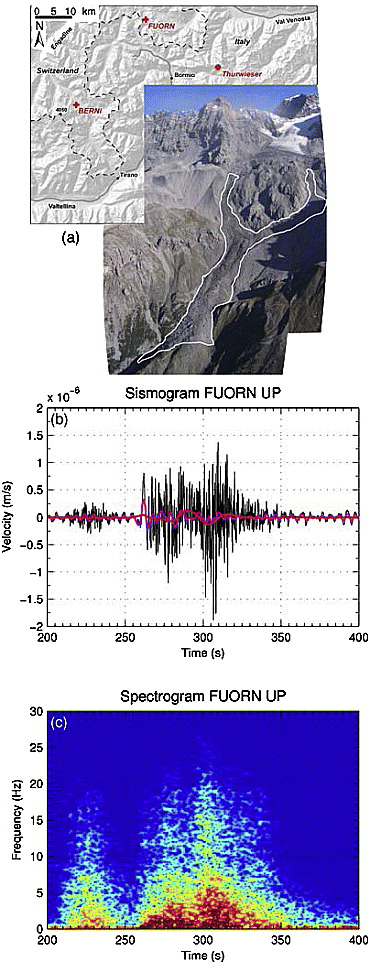
Fig. 1 - (a) Map showing the location of the Thurwieser rock avalanche (Italy) and the FUORN and BERNI seismic stations (Switzerland). The picture shows the rock avalanche deposit [Sosio et al., 2008] outlined with white dashed lines for thicknesses h > 1 m. (b) Vertical ground velocity recorded at FUORN station. The recorded seismic signal is represented in black for the raw data and in pink and red for the data filtered at 5–20 s and 20–50 s, respectively. (c) Spectrogram of the seismic signal.

The seismic signal generated by the rock avalanche was recorded by two broadband Streckeisen STS-2 seismic stations, FUORN (N46.62, E10.26) and BERNI (N46.41, E10.02), located in Switzerland at about 24 km and 39 km from the source, respectively. The vertical ground velocity was ∼1 × 10−6 m s^-1 at FUORN and the duration of the seismic signal was about 150 s with a main frequency range f ∈ [0, 10] Hz (Figures 1b and 1c). An initial small amplitude signal lasting 50 s, possibly due to rockfall activity, was observed just before the rock avalanche started to flow [Sosio et al., 2008]. It was followed by a strong signal observed for about 90 s (roughly the landslide duration) with a larger low frequency content, mainly made of a small pulse followed by two higher amplitude pulses (Figures 1b, 1c, and 3).

3. Landslide Simulation

The idea is to calculate the spatio-temporal stress field representing the low frequency source function of “landquakes” using classical avalanche models. The Thurwieser landslide has already been simulated with calibration of the rheological parameters using unique front velocity data [Sosio et al., 2008]. Generally models are calibrated using the runout distance and, when available, the deposit extent. However these data are hardly ever measured for natural events, in particular for submarine landslides. We show here that models can be calibrated using the seismic signal generated by the landslide, a measurement that can easily be obtained from seismic networks and that contains information on the dynamics.

We use here the SHALTOP numerical model that describes granular flows over a complex 3D topography [Bouchut et al., 2003; Bouchut and Westdickenberg, 2004; Mangeney-Castelnau et al., 2005; Mangeney et al., 2007a]. This model is based on the depth-averaged thin layer approximation and takes into account a Coulomb type friction law. It describes the change in time of the thickness h(x, y, t) in the direction normal to the topography and of the depth-averaged velocity of the flow u(x, y, t) along the topography z = b(x, y), where (x, y, z) are the coordinates in a horizontal/vertical reference frame. Contrary to most models used in geophysics, this model deals with the full tensor of terrain curvature equation image. SHALTOP has successfully reproduced experimental granular flows [Mangeney-Castelnau et al., 2005; Mangeney et al., 2007a] and natural landslides [Lucas and Mangeney, 2007; Kuo et al., 2009].

As the main issue in landslide modeling is their still unknown mechanical behaviour, we choose the simplest friction law involving only one empirical parameter, the friction coefficient μ = tan δ, where δ is the friction angle. This parameter can be considered as a measure of the mean dissipation during the flow. The material involved in the Thurwieser avalanche mainly consists of dry, broken rocks mixed with a few ice blocks so that an empirical friction coefficient typical of dry granular flows is expected. Note that for natural landslides with volumes ≥1 Mm³, the empirical friction angle δ is generally smaller than the typical friction angle of natural material (δn ≥ 30°) [e.g., Pirulli and Mangeney, 2008].

We performed numerical simulations using the pre- and post-event Digital Elevation Model provided by Sosio et al. [2008]. The friction angles were calibrated to best fit the observed runout distance. Assuming a constant friction coefficient over the entire avalanche path, the best fit of the runout distance was obtained with δ = 23° (Figures 2a–2c). In that case, hereafter called scenario 1, the main part of the mass stops on the plateau covered by the glacier, before the headwall, with a maximum deposit thickness of 43 m and a thin deposit (h < 12 m) in the downslope valley. The maximum velocity below the glacier is about 50 m s^-1, reached at time t ≃ 45 s when the front descends the headwall. The upper part of the flow stops at ts ≃ 45 s while the remaining mass located downslope within the valley stops at around ts = 100 s.

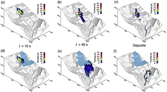
Fig. 2 - Numerical modeling of the Thurwieser rock avalanche (a–c) without taking the glacier into account, i.e., with a constant friction angle δ = 23°, and (d–f) taking the glacier into account with friction angles δ1 = 26°, and δ2 = 6° when the mass flows over the glacier (represented in light blue).

However, the presence of a glacier along the avalanche path is known to significantly reduce the basal friction when the flow passes over it [Sosio et al., 2008]. The simplest way to take this into account is to assign a different friction angle for flow over the glacier, i.e., δ2, while the friction angle is δ1 everywhere else. The observed runout distance can be reproduced numerically with various combinations of (δ1, δ2). The results are shown in Figures 2d–2f for friction angles δ1 = 26° and δ2 = 6°, hereafter referred to as scenario 2, that give the best fit to the seismic signal (see section 5). In this case, the dynamics are very different from scenario 1. Due to the low friction on the glacier, the main part of the mass overrides and spreads out widely over the headwall. The bulk deposit is found downslope in the Marè valley with maximum thickness of 27.5 m, in agreement with field observations [Sosio et al., 2008] (Figures 1a and 2f). The maximum velocity downslope of the glacier is about 65 m s^-1, reached at time t ≃ 40 s when the front descends the headwall, also consistent with field measurements, showing that calibration using the seismic signal helps constrain the flow dynamics. The mass stops at time ts ≃ 100 s.

4. Landquake Seismic Wave Modeling

The flowing mass generates a time dependent basal stress field applied on top of the terrain, inducing seismic waves. In the topographic reference frame ($e_X$, $e_Y$, $e_Z$), where $e_Z$ is directed upwards normal to the plane tangent to the topography and ($e_X$, $e_Y$) defines an orthonormal reference frame in this plane, the stress T = ($T_X, T_Y, T_Z$) can be expressed as:

\begin{equation} T = \rho g h \left( \cos \theta + \frac{u^t_h H u_h}{g \cos^3\theta} \right) \left(\mu \frac{x}{\| u \|},\mu \frac{u_y}{\| u \|},-1 \right), \end{equation}

where θ(x, y) is the steepest slope angle, $u_h$ = ($u_x$, $u_y$) the projection of the velocity in the horizontal plane, g acceleration due to gravity and ρ the density of the flowing mass. Equation (1) shows that the simulated source essentially reflects the loading/unloading conditions related to the spatio-temporal variation of the thickness of the flowing mass which is in turn a result of a complex balance between inertia, pressure gradients, gravity and friction [Mangeney-Castelnau et al., 2003]. Centrifugal acceleration also contributes due to the curvature radii of the terrain (second term in expression (1)). The tangential stress involves the friction coefficient as defined by the Coulomb friction law.

The calculated stress field (1) is used as a surface boundary condition in a seismic wave propagation model. This model, developed by Pascal Favreau, is based on a fast Green's function calculation with a discrete frequency-wavenumber method inspired by the work of Bouchon [1979]. Here, topography and complex media effects are neglected and the model solves the elastodynamic equations in a horizontally stratified half-space. Free surface boundary conditions are applied at the top, continuity conditions at each interface and vanishing conditions at infinite depth.

Because depth-averaged landslide models like the one used here do not simulate high frequency sources related to impacts and collisions of individual blocks, only the long-period simulated and recorded seismic signals are compared, i.e., T ∈ [20 s, 50 s]. For T ≥ 20 s, the typical wavelength is λ = cT ≥ 50 km for a typical wave velocity of c = 2.5 km s^-1. In this frequency range, topographic and complex media effects are expected to weakly affect seismic wave propagation. Here, the source-seismometer distance is <40 km, so that for periods T ≥ 20 s the recorded seismic signal can be considered as a near-field signal.

5. Results

Let us compare the observed and simulated vertical components of the seismic signals at FUORN station, filtered between 20 s and 50 s, for scenario 1 and 2 (Figure 3a). The signal calculated using scenario 1 (without glacier) simulates the two first peaks observed in the data, however the last peak is not reproduced. The sign and amplitude of the first motion well match the data until tl = 20 s, where tl is counted from the beginning of the seismic signal t0 and roughly corresponds to the time elapsed from the initial mass destabilization. The simulation overestimates the amplitude for 20 s < tl < 45 s and underestimates it for tl > 50 s. Similar features are observed for BERNI station (Figure 3b).

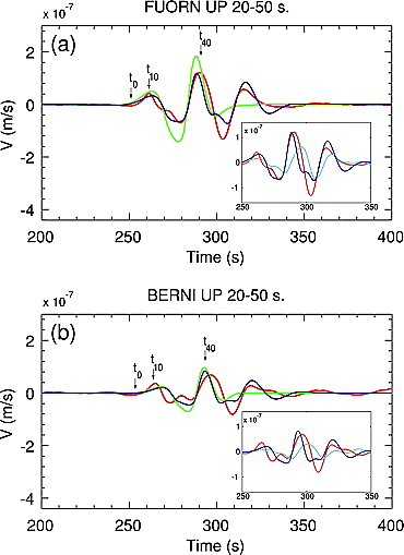
Fig. 3 - Vertical ground velocity filtered at 20–50 s at (a) FUORN and (b) BERNI stations. Observed data are represented in red and the seismic signal calculated from scenario 1 (without glacier) and scenario 2 (with glacier) are represented in green and blue, respectively. Inserts: comparison between observed data (red) and the seismic signals simulated with (dark blue) and without (light blue) curvature effects (see equation (1)).

Taking into account the glacier significantly improves the results: the simulated amplitude closely matches the data, and the last peak observed in the seismic signal is accurately reproduced for both stations (Figures 3a and 3b). The peak ground velocity is accurately simulated for both stations. The simulated amplitude is underestimated only for 50 s < tl < 60 s. Analysis of the horizontal components give similar qualitative results but less agreement between simulated and observed signals.

These results show that the landslide dynamics are much better reproduced using scenario 2. Although analysis of the seismic signal in terms of flow dynamics is relatively uncertain, we propose some possible interpretations of the results. At the beginning (tl < 20 s), the simulated seismic signal is almost the same for the two scenarios that differ only in terms of the values of the friction coefficients. This may result from the small contribution of the friction force compared to inertia or longitudinal pressure gradients, during the first instants of a granular mass collapse [e.g., Mangeney-Castelnau et al., 2003]. Due to the low friction angle when the landslide passes over the glacier, the mass spreads over the entire headwall in scenario 2 while it is restricted to a narrow zone in scenario 1 (Figures 2e and 2b). The larger spreading observed in scenario 2 at time 20 s < tl < 45 s is associated with smaller amplitude seismic signals. At tl > 50–55 s in scenario 1, the main part of the mass is already at rest upslope while a small amount of material is still flowing in the valley below, contrary to scenario 2 where the entire mass is flowing in the valley, generating a higher amplitude seismic signal. A sensitivity study has been performed by varying the friction angles in the model. The best fit for the seismic signal is obtained for friction coefficients δ1 = 26° and δ2 = 6° (see section 3). These friction angles are similar to those fitted for front velocity data by Sosio et al. [2008].

Curvature effects play a major role in the generated seismic signal. Indeed, the signal simulated without taking into account the curvature term does not fit the data (inserts in Figure 3). Numerical simulation clearly shows that the sensitivity of the flow to the topography strongly depends on its rheology. Because the dynamics of the flow over the topography is “scanned” by the seismic signal, the signal can be analyzed to recover the flow history and thus the rheological parameters, if topography effects are accounted for.

6. Conclusion

The simulation of a landslide and the generated seismic waves is shown to explain the main features of landquake low frequency seismic signals observed at distances greater than about 10 times the length of the landslide. We show here that the effects of topography on the flowing mass have a major impact on the generated seismic signal, as already suggested by Suriñach et al. [2001]. As a result, analysis of the seismic signal must take into account the complex 3D topography along the avalanche path. On the other hand, for the source-station distance and periods considered here, topography seems to only weakly affect wave propagation.

We have shown that the seismic signal can be used to calibrate the rheological parameters characterizing the flow. As seismic waves reflect the flow dynamics, they provide stronger constraints on the rheological parameters than information on the deposit which, in addition, is not always available [e.g., Mangeney-Castelnau et al., 2005].

This is a very important result given that seismic signals generated by landslides of significant size are recorded by local or regional permanent seismic networks providing unique data on natural flow dynamics. The seismic signal generated by landslides can be analyzed to provide new data on the time duration and mobility of natural flows that may help improve our understanding of their yet unexplained high mobility. As erosion processes or fluid/solid interactions have been shown to significantly change flow dynamics [e.g., Iverson, 1997; Hungr and Evans, 2004; Mangeney et al., 2007b, 2010; Crosta et al., 2009], there is some hope of recovering the signature of these processes through detailed analysis of the generated seismic signals.

Much more work needs to be done to systematically quantify the effects of the initial geometry and volume of the released mass, topography and rheological parameters on the generated seismic signal. Furthermore detailed analysis of the effect of topography and complex media on wave propagation depending on the landquake-station distance must be investigated.

References

Bouchut, F., A. Mangeney-Castelnau, B. Perthame, and J. P. Vilotte (2003), A new model of Saint-Venant and Savage-Hutter type for gravity driven shallow water flows, C. R. Acad. Sci. Paris, Ser. I, 336, 531–536.
Bouchut, F., and M. Westdickenberg (2004), Gravity driven shallow water models for arbitrary topography, Commun. Math. Sci, 2, 359–389.
Brodsky, E. E., E. Gordeev, and H. Kanamori (2003), Landslide basal friction as measured by seismic waves, Geophys. Res. Lett., 30(24), 2236, doi:10.1029/2003GL018485.
Cole, S. E., S. J. Cronin, S. Sherburn, and V. Manville (2009), Seismic signals of snow-slurry lahars in motion: 25 September 2007, Mt Ruapehu, New Zealand, Geophys. Res. Lett., 36, L09405, doi:10.1029/2009GL038030.
Crosta, G. B., S. Imposimato, and D. Roddeman (2009), Numerical modeling of 2-D granular step collapse on erodible and nonerodible surface, J. Geophys. Res., 114, F03020, doi:10.1029/2008JF001186.
Dahlen, F. A. (1993), Single-force representation of shallow landslide sources, Bull. Seismol. Soc. Am., 83(1), 130–143.
De Angelis, S., V. Bass, V. Hards, and G. Ryan (2007), Seismic characterization of pyroclastic flow activity at Soufrière Hills Volcano, Montserrat, Nat. Hazards Earth Syst. Sci., 7, 467–472.
Deparis, J., D. Jongmans, F. Cotton, L. Baillet, F. Thouvenot, and D. Hantz (2008), Analysis of rock-fall and rock-fall avalanche seismograms in the French Alps, Bull. Seismol. Soc. Am., 98(4), 1781–1796.
Huggel, C., J. Caplan-Auerbach, C. F. Waythomas, and R. L. Wessels (2007), Monitoring and modeling ice-rock avalanches from ice-capped volcanoes: A case study of frequent large avalanches on Iliamna Volcano, Alaska, J. Volcanol. Geotherm. Res., 168(1–4), 114–136.
Hungr, O., and S. G. Evans (2004), Entrainment of debris in rock avalanches: An analysis of a long run-out mechanism, Bull. Geol. Soc. Am., 9–10(116), 1240–1252.
Iverson, R. M. (1997), The physics of debris flows, Rev. Geophys., 35, 245–296.
Kishimura, K., and K. Izumi (1997), Seismic signals induced by snow avalanche flow, J. Nat. Hazards, 15(1), 89–100.
Kuo, C. Y., Y. C. Tai, F. Bouchut, A. Mangeney, M. Pelanti, R. F. Chen, and K. J. Chang (2009), Simulation of Tsaoling Landslide, Taiwan, based on Saint Venant equations over general topography, Eng. Geol., 104(3–4), 181–189.
La Rocca, M., D. Galluzzo, G. Saccorotti, S. Tinti, G. B. Cimini, and E. Del Pezzo (2004), Seismic signals associated with landslides and with a tsunami at Stromboli Volcano, Italy, Bull. Seismol. Soc. Am., 94(5), 1850–1867.
Legros, F. (2002), The mobility of long-runout landslides, Eng. Geol., 63, 301–331.
Lucas, A., and A. Mangeney (2007), Mobility and topographic effects for large Valles Marineris landslides on Mars, Geophys. Res. Lett., 34, L10201, doi:10.1029/2007GL029835.
Mangeney, A., L. S. Tsimring, D. Volfson, I. S. Aranson, and F. Bouchut (2007a), Avalanche mobility induced by the presence of an erodible bed and associated entrainment, Geophys. Res. Lett., 34, L22401, doi:10.1029/2007GL031348.
Mangeney, A., F. Bouchut, N. Thomas, J. P. Vilotte, and M. O. Bristeau (2007b), Numerical modeling of self-channeling granular flows and of their levee-channel deposits, J. Geophys. Res., 112, F02017, doi:10.1029/2006JF000469.
Mangeney, A., O. Roche, O. Hungr, N. Mangold, G. Faccanoni, and A. Lucas (2010), Erosion and mobility in granular collapse over sloping beds, J. Geophys. Res., doi:10.1029/2009JF001462, in press.
Mangeney-Castelnau, A., J.-P. Vilotte, M. O. Bristeau, B. Perthame, F. Bouchut, C. Simeoni, and S. Yerneni (2003), Numerical modeling of avalanches based on Saint Venant equations using a kinetic scheme, J. Geophys. Res., 108(B11), 2527, doi:10.1029/2002JB002024.
Mangeney-Castelnau, A., F. Bouchut, J. P. Vilotte, E. Lajeunesse, A. Aubertin, and M. Pirulli (2005), On the use of Saint Venant equations to simulate the spreading of a granular mass, J. Geophys. Res., 110, B09103, doi:10.1029/2004JB003161.
Pirulli, M., and A. Mangeney (2008), Result of back-analysis of the propagation of rock avalanches as a function of the assumed rheology, Rock Mech. Rock Eng., 41(1), 59–84.
Sosio, R., G. B. Crosta, and O. Hungr (2008), Complete dynamic modeling calibration for the Thurwieser rock avalanche (Italian Central Alps), Eng. Geol., 100(1–2), 11–26.
Suriñach, E., G. Furdada, F. Sabot, B. Biescas, and J. M. Vilaplana (2001), On the characterization of seismic signals generated by snow avalanches for monitoring purposes, Ann. Glaciol., 32(1) 268–274.
Vilajosana, I., E. Suriñach, G. Khazaradze, and P. Gauer (2007), Snow avalanche energy estimation from seismic signal analysis, Cold Reg. Sci. Technol., 50(1–3), 72–85.